
Python Pandas Module
- Pandas is an open source library in Python. It provides ready to use high-performance data structures and data analysis tools.
- Pandas module runs on top of NumPy and it is popularly used for data science and data analytics.
- NumPy is a low-level data structure that supports multi-dimensional arrays and a wide range of mathematical array operations. Pandas has a higher-level interface. It also provides streamlined alignment of tabular data and powerful time series functionality.
- DataFrame is the key data structure in Pandas. It allows us to store and manipulate tabular data as a 2-D data structure.
- Pandas provides a rich feature-set on the DataFrame. For example, data alignment, data statistics, slicing, grouping, merging, concatenating data, etc.
Installing and Getting Started with Pandas
You need to have Python 2.7 and above to install Pandas module. If you are using conda, then you can install it using below command.
conda install pandas
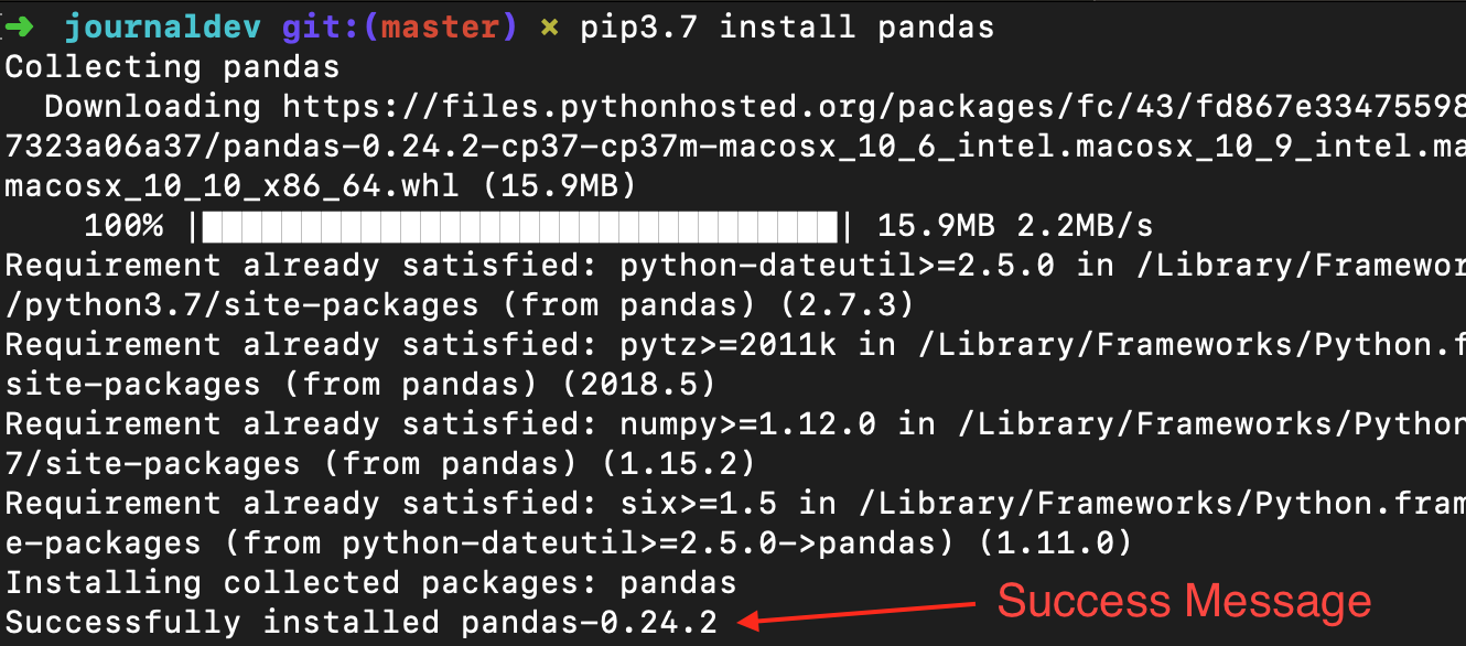
If you are using PIP, then run the below command to install pandas module.
pip3.7 install pandas
To import Pandas and NumPy in your Python script, add the below piece of code:
import pandas as pd
import numpy as np
As Pandas is dependent on the NumPy library, we need to import this dependency.
Data Structures in Pandas module
There are 3 data structures provided by the Pandas module, which are as follows:
- Series: It is a 1-D size-immutable array like structure having homogeneous data.
- DataFrames: It is a 2-D size-mutable tabular structure with heterogeneously typed columns.
- Panel: It is a 3-D, size-mutable array.
Pandas DataFrame
DataFrame is the most important and widely used data structure and is a standard way to store data. DataFrame has data aligned in rows and columns like the SQL table or a spreadsheet database. We can either hard code data into a DataFrame or import a CSV file, tsv file, Excel file, SQL table, etc. We can use the below constructor for creating a DataFrame object.
pandas.DataFrame(data, index, columns, dtype, copy)
Below is a short description of the parameters:
- data - create a DataFrame object from the input data. It can be list, dict, series, Numpy ndarrays or even, any other DataFrame.
- index - has the row labels
- columns - used to create column labels
- dtype - used to specify the data type of each column, optional parameter
- copy - used for copying data, if any
There are many ways to create a DataFrame. We can create DataFrame object from Dictionaries or list of dictionaries. We can also create it from a list of tuples, CSV, Excel file, etc. Let’s run a simple code to create a DataFrame from the list of dictionaries.
import pandas as pd
import numpy as np
df = pd.DataFrame({
    "State": ['Andhra Pradesh', 'Maharashtra', 'Karnataka', 'Kerala', 'Tamil Nadu'],
    "Capital": ['Hyderabad', 'Mumbai', 'Bengaluru', 'Trivandrum', 'Chennai'],
    "Literacy %": [89, 77, 82, 97,85],
    "Avg High Temp(c)": [33, 30, 29, 31, 32 ]
})
print(df)
Output:  The first step is to create a dictionary. The second step is to pass the dictionary as an argument in the DataFrame() method. The final step is to print the DataFrame. As you see, the DataFrame can be compared to a table having heterogeneous value. Also, the size of the DataFrame can be modified. We have supplied the data in the form of the map and the keys of the map are considered by Pandas as the row labels. The index is displayed in the leftmost column and has the row labels. The column header and data are displayed in a tabular fashion. It is also possible to create indexed DataFrames. This can be done by configuring the index parameter in the
 DataFrame() method.
Importing data from CSV to DataFrame
We can also create a DataFrame by importing a CSV file. A CSV file is a text file with one record of data per line. The values within the record are separated using the “comma” character. Pandas provides a useful method, named read_csv() to read the contents of the CSV file into a DataFrame. For example, we can create a file named ‘cities.csv’ containing details of Indian cities. The CSV file is stored in the same directory that contains Python scripts. This file can be imported using:
import pandas as pd
data =  pd.read_csv('cities.csv')
print(data)
. Our aim is to load data and analyze it to draw conclusions. So, we can use any convenient method to load the data. In this tutorial, we are hard-coding the data of the DataFrame.
Inspecting data in DataFrame
Running the DataFrame using its name displays the entire table. In real-time, the datasets to analyze will have thousands of rows. For analyzing data, we need to inspect data from huge volumes of datasets. Pandas provide many useful functions to inspect only the data we need. We can use df.head(n) to get the first n rows or df.tail(n) to print the last n rows. For example, the below code prints the first 2 rows and last 1 row from the DataFrame.
print(df.head(2))
Output: 
print(df.tail(1))
Output:  Similarly,
 print(df.dtypes) prints the data types. Output: 
print(df.index) prints index. Output: 
print(df.columns) prints the columns of the DataFrame. Output: 
print(df.values) displays the table values. Output: 
1. Getting Statistical summary of records
We can get statistical summary (count, mean, standard deviation, min, max etc.) of the data using df.describe() function. Now, let’s use this function, to display the statistical summary of “Literacy %” column. To do this, we may add the below piece of code:
print(df['Literacy %'].describe())
Output:  The
The df.describe() function displays the statistical summary, along with the data type.
2. Sorting records
We can sort records by any column using df.sort_values() function. For example, let’s sort the “Literacy %” column in descending order.
print(df.sort_values('Literacy %', ascending=False))
Output: 
3. Slicing records
It is possible to extract data of a particular column, by using the column name. For example, to extract the ‘Capital’ column, we use:
df['Capital']
or
(df.Capital)
Output:  It is also possible to slice multiple columns. This is done by enclosing multiple column names enclosed in 2 square brackets, with the column names separated using commas. The following code slices the ‘State’ and ‘Capital’ columns of the DataFrame.
print(df[['State', 'Capital']])
Output:  It is also possible to slice rows. Multiple rows can be selected using “:” operator. The below code returns the first 3 rows.
df[0:3]
Output:  An interesting feature of Pandas library is to select data based on its row and column labels using
 iloc[0] function. Many times, we may need only few columns to analyze. We can also can select by index using loc['index_one']). For example, to select the second row, we can use df.iloc[1,:] . Let’s say, we need to select second element of the second column. This can be done by using df.iloc[1,1] function. In this example, the function df.iloc[1,1] displays “Mumbai” as output.
4. Filtering data
It is also possible to filter on column values. For example, below code filters the columns having Literacy% above 90%.
print(df[df['Literacy %']>90])
Any comparison operator can be used to filter, based on a condition. Output:  Another way to filter data is using the
 isin. Following is the code to filter only 2 states ‘Karnataka’ and ‘Tamil Nadu’.
print(df[df['State'].isin(['Karnataka', 'Tamil Nadu'])])
Output: 
5. Rename column
It is possible to use the df.rename() function to rename a column. The function takes the old column name and new column name as arguments. For example, let’s rename the column ‘Literacy %’ to ‘Literacy percentage’.
df.rename(columns = {'Literacy %':'Literacy percentage'}, inplace=True)
print(df.head())
The argument `inplace=True` makes the changes to the DataFrame. Output: 
6. Data Wrangling
Data Science involves the processing of data so that the data can work well with the data algorithms. Data Wrangling is the process of processing data, like merging, grouping and concatenating. The Pandas library provides useful functions like merge(), groupby() and concat() to support Data Wrangling tasks. Let’s create 2 DataFrames and show the Data Wrangling functions to understand it better.
import pandas as pd

d = {
    'Employee_id': ['1', '2', '3', '4', '5'],
    'Employee_name': ['Akshar', 'Jones', 'Kate', 'Mike', 'Tina']
}
df1 = pd.DataFrame(d, columns=['Employee_id', 'Employee_name'])
print(df1)
Output:  Let’s create the second DataFrame using the below code:
import pandas as pd

data = {
    'Employee_id': ['4', '5', '6', '7', '8'],
    'Employee_name': ['Meera', 'Tia', 'Varsha', 'Williams', 'Ziva']
}
df2 = pd.DataFrame(data, columns=['Employee_id', 'Employee_name'])
print(df2)
Output: 
a. Merging
Now, let’s merge the 2 DataFrames we created, along the values of ‘Employee_id’ using the merge() function:
print(pd.merge(df1, df2, on='Employee_id'))
Output:  We can see that merge() function returns the rows from both the DataFrames having the same column value, that was used while merging.
b. Grouping
Grouping is a process of collecting data into different categories. For example, in the below example, the “Employee_Name” field has the name “Meera” two times. So, let’s group it by “Employee_name” column.
import pandas as pd
import numpy as np

data = {
    'Employee_id': ['4', '5', '6', '7', '8'],
    'Employee_name': ['Meera', 'Meera', 'Varsha', 'Williams', 'Ziva']
}
df2 = pd.DataFrame(data)

group = df2.groupby('Employee_name')
print(group.get_group('Meera'))
The ‘Employee_name’ field having value ‘Meera’ is grouped by the column “Employee_name”. The sample output is as below: Output: 
c. Concatenating
Concatenating data involves to add one set of data to other. Pandas provides a function named concat() to concatenate DataFrames. For example, let’s concatenate the DataFrames df1 and df2 , using :
print(pd.concat([df1, df2]))
Output: 
Create a DataFrame by passing Dict of Series
To create a Series, we can use the pd.Series() method and pass an array to it. Let’s create a simple Series as follows:
series_sample = pd.Series([100, 200, 300, 400])
print(series_sample)
Output:  We have created a Series. You can see that 2 columns are displayed. The first column contains the index values starting from 0. The second column contains the elements passed as series. It is possible to create a DataFrame by passing a dictionary of `Series`. Let’s create a DataFrame that is formed by uniting and passing the indexes of the series. Example
d = {'Matches played' : pd.Series([400, 300, 200], index=['Sachin', 'Kohli', 'Raina']),
'Position' : pd.Series([1, 2, 3, 4], index=['Sachin', 'Kohli', 'Raina', 'Dravid'])}
df = pd.DataFrame(d)
print(df)
Sample output  For series one, as we have not specified label ‘d’, NaN is returned.
Column Selection, Addition, Deletion
It is possible to select a specific column from the DataFrame. For example, to display only the first column, we can re-write the above code as:
d = {'Matches played' : pd.Series([400, 300, 200], index=['Sachin', 'Kohli', 'Raina']),
 'Position' : pd.Series([1, 2, 3, 4], index=['Sachin', 'Kohli', 'Raina', 'Dravid'])}
df = pd.DataFrame(d)
print(df['Matches played'])
The above code prints only the “Matches played” column of the DataFrame. Output  It is also possible to add columns to an existing DataFrame. For example, the below code adds a new column named “Runrate” to the above DataFrame.
d = {'Matches played' : pd.Series([400, 300, 200], index=['Sachin', 'Kohli', 'Raina']),
 'Position' : pd.Series([1, 2, 3, 4], index=['Sachin', 'Kohli', 'Raina', 'Dravid'])}
df = pd.DataFrame(d)
df['Runrate']=pd.Series([80, 70, 60, 50], index=['Sachin', 'Kohli', 'Raina', 'Dravid'])
print(df)
Output:  We can delete columns using the `delete` and `pop` functions. For example to delete the ‘Matches played’ column in the above example, we can do it by either of the below 2 ways:
del df['Matches played']
or
df.pop('Matches played')
Output: 
Conclusion
In this tutorial, we had a brief introduction to the Python Pandas library. We also did hands-on examples to unleash the power of the Pandas library used in the field of data science. We also went through the different Data Structures in the Python library. Reference: Pandas Official Website
Thanks for learning with the DigitalOcean Community. Check out our offerings for compute, storage, networking, and managed databases.
author


Get our biweekly newsletter
Sign up for Infrastructure as a Newsletter.

Hollie's Hub for Good
Working on improving health and education, reducing inequality, and spurring economic growth? We'd like to help.

Become a contributor
Get paid to write technical tutorials and select a tech-focused charity to receive a matching donation.

Thanks for your Tutorials about simple basic data analysis it is very help to understand better of AI
- Ferdy